overview
Mastering the Dash 2 Trade Backtester: A Step-by-Step Guide (Beta Version)
Introduction
Introducing the Dash 2 Trade backtester, your gateway to unlocking trading success.
This user-friendly tool enables you to harness the power of backtesting with its intuitive interface and comprehensive features. With three key sections at your disposal, you can effortlessly navigate through the backtesting process. In the "Select Asset" section, choose your desired asset, timeframe, and date range to set the stage for your backtest. Next, dive into the "Triggers & Conditions" section, where you’ll create your trading logic and bring indicators to life. Finally, in the "Settings" section, fine-tune your strategies, set risk parameters, and optimize your approach.
Get ready to embark on a journey of discovery and growth as a trader with the Dash 2 Trade backtester.
But first …
What Is a Backtester?
A backtester is a fantastic tool that can give traders a deeper understanding of the advantages and shortfalls of their chosen trading strategy. Backtesters use historical price data to simulate trades over a period of time, based on user-defined conditions (i.e., your strategy).
Once the simulation is finished the user can review it to see under what historical market conditions their strategy would have been successful and where it would have been less so.
First Steps: Overview
To access the backtester, simply navigate to the left side menu and locate the "Tools" section. Within this section, you'll find the option labeled "Backtester," as shown in the image below. Click on it to enter the backtester.

If you"re new to the backtester, here is the initial screen you will encounter:

To create a strategy, simply click on the "+ Create Strategy" button.
You will be redirected to a screen where you will see 3 sections:
- Select Asset
- Triggers & Conditions
- Settings
Select Asset: Your Trading Playground
Welcome to the heart of the Dash 2 Trade backtester! This is where your trading journey begins.
In this section, you have the power to select the asset you want to trade, choose the timeframe that suits your trading style, and set the range of dates for the backtest. It's your playground to explore, analyze, and unleash your trading potential.

Triggers & Conditions: Unleash Your Trading Magic
Now it's time to unlock the magic of your trading strategies. In this section, you'll create the logic that drives your trading decisions.
You will start by defining your entry and exit conditions, both for long and short positions, to capture those profitable opportunities. The user-friendly interface requires absolutely no coding, allowing you to experiment with conditions quickly and build the foundation for your successful trades.
Settings: Fine-Tune Your Strategy
Here's where you can fine-tune your strategy and take control of your risk management.
You can set your desired take-profit and stop-loss thresholds as percentages, to secure your gains and protect against potential losses. Additionally, you have the option to define limits for daily and weekly profit and loss to stay within your desired risk tolerance. While not mandatory, these settings allow you to optimize your strategies and align them with your specific goals.
Note: Stay tuned for upcoming engine settings that will further enhance your trading experience.

With the Dash 2 Trade backtester, you have a powerful tool at your fingertips. It's time to unleash your trading magic, fine-tune your strategies, and embark on a journey toward trading success. Get ready to experience the world of backtesting like never before. Let's take your trading to new heights!
Getting Started: Selecting Assets, Timeframes, and Dates

Selecting The Token
This is the first step of the backtesting process, where you choose the asset you want to trade. By clicking on the token dropdown menu, you can easily select the desired coin for testing. Alternatively, you can directly enter the symbol of the coin or asset. If it is available, it will appear in the dropdown menu.

Note: Please be aware that stablecoins and wrapped tokens may also be displayed in the menu. However, we recommend avoiding them as target coins for testing purposes.
Selecting Timeframe
Once you have selected the target coin, the next step is to choose the timeframe.
Note: In this Beta Version, the backtester will run using the timeframe defined in the logic. In future versions of the backtester, there will be a separate section dedicated to selecting logic assets and timeframes, allowing for multi-timeframe and cross-asset capabilities.
Here is the menu where you can conveniently choose the timeframe that best suits your testing needs:

Selecting Start & End Dates
Choosing the start and end dates for your backtest is a crucial step in the process. By default, the backtester displays today's date as the end date and sets the start date to three years prior. This three-year window strikes a balance between having enough historical data for analysis and avoiding potential biases or overfitting. However, users have the flexibility to select their preferred dates, enabling them to test different ranges of dates and gain insights from different perspectives.
Selecting the desired start and end dates is a straightforward process. The backtester employs a user-friendly calendar format, similar to what you may have encountered on other platforms. This intuitive interface allows you to easily navigate through the available dates and pinpoint the specific timeframe you wish to analyze.

Important: It"s important to note that the backtester requires a minimum of two days worth of data to perform a meaningful analysis. Therefore, when selecting dates, please ensure that the chosen time frame spans at least three days in order to obtain reliable results.
Defining Trading Logic and Indicators
Let's discuss how to define the trading logic to be tested.
Note: By “logic” we mean the conditions that dictate what the backtester will simulate (i.e., when to buy and when to sell).
Overview
To grasp the construction of the logic, it’s important to understand how certain elements work. The backtester’s logic set determines when to open or close a position based on specific conditions. When the logic set returns true at a particular point in the data time series, the action is executed at the next opening price, except in cases where the trigger is a take-profit or sell-loss. In these instances, the take-profit or sell-loss is triggered in the same data point, without waiting for the next opening price.
Now let's explore the heart of the backtester, which revolves around logical operators comparing two values. The logic is divided into two categories: long-position logic and short-position logic. A long position involves buying an asset with the expectation of its value increasing, while a short position involves selling an asset with the anticipation of its price decreasing.

Within the process of constructing the logic, whether it is for a long or short position, there are two key components:
- the logic for opening a position
- and the logic for closing a position.
These components allow you to define when the backtester will enter and exit a trade.
As shown in the image below, the opening logic is located on the left side, while the closing logic is positioned on the right side. This clear visual separation allows for easy distinction between the two components, facilitating the design and understanding of the trading strategy.

The logic construction involves selecting Open, High, Low, Close, and Volume (OHLCV) data or selecting indicators using dropdown menus on both sides. The logic symbols ">" and "<" are used to compare the logic pair.

For example, if you select "high" in the first dropdown menu and "open" in the second dropdown menu, and then choose the logic symbol ">", it means that you will have "high" ">" "open", which can be interpreted as:
“when the “high” value “is greater than” the “open” value…”

Logic Building - Building Simple Logic
Now that we have gained a basic understanding of how the logic works, let's delve into constructing logic for a simple strategy.
In this example, we will use the following condition: If the price is above the 20-period exponential moving average (EMA), we will enter a long position. If the price is below the 20-period EMA, we will close the long position and initiate a short position.
This straightforward logic will serve as a starting point to demonstrate the process of building strategies within the backtester.
Adding Indicator
Let's start from the beginning. When you click on the "indicator" dropdown menu, you will see several options to choose from: "open price", "high price", "low price", "close price", "volume", and "rv".

The options with "price" in their names are related to the different components of a candle in a time series.
If you’re unfamiliar with the concept of a trading candle, we recommend taking a moment to understand it fully before proceeding.
"Volume" represents the trading volume expressed in USDT, not the number of tokens/coins traded. Lastly, "rv" stands for "realized volatility," which is a measurement of volatility that we use on outlier events within the platform.
Understanding these different options will be crucial as we build our logic and select the appropriate indicators to create our trading strategy. Don't worry if you’re not familiar with all the terms right away. We’ll guide you through the process and explain the concepts along the way to ensure a smooth learning experience.
As mentioned, the dropdown menu doesn’t contain the indicators themselves. Instead, you’ll find a "+ Add New Indicator" button.

Clicking on this button will open a new window where you can choose the specific indicator you want to use. This window presents a selection of indicators for you to explore and utilize in your strategy.


You can select indicators based on your preferred trading strategies and the specific insights you want to gain from the backtesting process. It’s an opportunity to tailor your logic to the indicators that best suit your needs and align with your trading style. But at this moment we will choose "EMA" which is an exponential moving average, to continue with the step-by-step.

When you click on "EMA" in the indicator selection window, a new window will appear. This window is now showing the configuration for the Exponential Moving Average (EMA) indicator. By default, the EMA parameters use the close price and 20 periods but you can adjust them as you wish.
You have the flexibility to add multiple indicators simultaneously. You can either click on "Apply" after configuring the EMA indicator to add it to your logic, or you can click on "+ Add Indicator" to add multiple indicators at once. This allows you to customize your strategy by incorporating different indicators and adjusting their parameters according to your trading preferences.
For now, we will click on Apply, after this, the logic will look like this:

For learning purposes, we will look into the first drop-down menu and see that the indicator is now to be chosen.

Now let’s finish our first logic pair, select "close price" and your EMA and it will look like this:

As you can see, we have:
"close price" ">" "EMA(close price, 20)"
Which means:
close price greater than "EMA(close price, 20)
Since we are not using any take-profit or sell-loss level (section 4), we will use the inverse logic to create the close-long position logic. The close logic will look like this:
After building the long logic, we will proceed to the short logic, to access the short logic you have to click on the “Short” button on the right side of the green button “Long”:

For the short position logic, we will simply invert the logic, in long we have:
- Open: close price greater than "EMA(close price, 20)
- Close: close price lesser than "EMA(close price, 20)
So, for short we will have:
- Open: close price lesser than "EMA(close price, 20)
- Close: close price greater than "EMA(close price, 20)
After setting the logic, click on “Next” and then “Save”. (This time we will skip the settings)
At this point you are ready to run your first backtest, it will be available in your backtest section like this:
After clicking on the “Run” button, you will have your backtest results for this simple strategy, on your screen, if everything runs ok you will see something like this:

Note: For now, we will skip the explanation of the results since this section is dedicated to logic building.
Logic Building - Adding Layers and Understanding how the components are put together.
After presenting a simple strategy, let's delve into how the logic set works. In the previous example, we used a single logic set with only one condition. However, it’s important to understand that there are different ways of constructing logic, which can yield different results.
Here is a good time to explain some concepts of logic, in the previous example we used:
LONG:
- Open: close price greater than "EMA(close price, 20)
- Close: close price lesser than "EMA(close price, 20)
SHORT:
- Open: close price lesser than "EMA(close price, 20)
- Close: close price greater than "EMA(close price, 20)
Now, let's explore how to add another layer to the logic by incorporating an additional indicator. In this example, we will introduce a 200-period Exponential Moving Average (EMA) alongside the existing 20-period EMA condition.

To add another condition to the logic, follow these steps:
- Click on the "+ Add Condition" button.
- A new condition will appear, allowing you to add another component to the logic.

Now, let's consider how to express this new condition to build the logical set. Before proceeding, make sure you have already created the 200-period EMA indicator (refer back to Section 3.2 for instructions).
Considering the first implementation for opening a long position:
"close price greater than "EMA(close price, 20)"
To incorporate the 200-period EMA, one might think of adding:
"close price greater than "EMA(close price, 200)"
Is this incorrect? No, but it depends on your specific trading strategy and objectives. Let’s explore the difference between two possible expressions:
Expression 1
"close price greater than EMA(close price, 20)"
and
"close price greater than EMA(close price, 200)"
Expression 2
"close price crosses up EMA(close price, 20)"
and
"close price greater than EMA(close price, 200)"
The key distinction lies in the condition used to compare the close price and the EMA indicator. In the first expression, we use the ">" (greater than) operator, while in the second expression, we use the "crosses up" operator.
In trading, these operators have different implications:
"close price greater than EMA(close price, 20)" and close price greater than EMA(close price, 200):
This condition is met when the close price is higher than both the 20-period and 200-period EMAs. It indicates a stronger bullish signal, suggesting an upward trend in the price. However, it doesn’t account for the specific moment of the price crossing above the 20-period EMA.
"close price crosses up EMA(close price, 20)" and close price greater than EMA(close price, 200):
This condition is met when the close price crosses above the 20-period EMA and is also higher than the 200-period EMA. It signifies a potential trend reversal and takes into account the specific moment when the price crosses above the 20-period EMA, indicating a bullish signal. This condition captures the momentum and can be interpreted as "when the long-term trend is bullish, if the price crosses above the 20-period EMA, I will buy."
The choice between these two expressions depends on your trading strategy and the specific signals you want to capture. By using the "crosses up" operator, you are considering the momentum and the occurrence of a specific event (i.e., the price crossing above the 20-period EMA). On the other hand, using only the "greater than" operator looks for a sustained bullish condition without considering the precise timing of the crossing event.
Understanding the different logic operators and their implications allows you to tailor your strategy to your trading style and preferences. By incorporating multiple indicators and employing various logic operators, you can create complex and sophisticated trading strategies within the backtester. This flexibility enables you to explore different combinations of indicators and conditions to refine your trading approach and enhance your overall trading performance.
Cross-UP & Cross-Down Operators
But now another question arises: among the possibilities in creating the logic, we only have the ">" operator, which means "greater than," and the "<" operator, which means "less than". If the "crosses up" operator does not appear when setting up a condition, how can we create this type of logic?
To create this logic, we can utilize a special indicator found in the "Special Operators" section. There, we will find the following options:
- LAG
- Cross-UP
- Cross-Down

By using these special operators, we can construct the desired logic.

The "cross-up" and "cross-down" operators rely on two inputs: the main value and the level. It is crucial to understand the distinction between these inputs, as their order matters. For instance, if you set the main value as the close price and the level as the 20-period exponential moving average (EMA), the "cross-up" operator detects when the close price crosses above the EMA 20, indicating a potentially bullish signal. However, if you reverse the inputs and set the EMA 20 as the main value and the close price as the level, the interpretation would be different. In this case, the "cross-up" operator would detect when the EMA 20 crosses above the close price, which may have a distinct meaning or implication. Therefore, it is essential to carefully designate the main value and the level, as their arrangement influences the logic and the resulting trading signals.
How to Use the Cross-up Operator in the Logic?
The cross-up/down operator offers a distinct advantage in strategy construction as it eliminates the requirement of using the ">" or "<" logic operators in combination with another value.
Let’s take a look at the visual representation below to understand how it functions:

As depicted in the image, the cross-up/down operator simplifies the logic by directly comparing the main value and the level without the need for additional comparison operators.
By incorporating this operator, we can easily set up the desired additional condition for our new test.

We have now reached a stage where we can create a trigger with two conditions, which has the potential to enhance our strategies.
To aid in our learning process, we will provide a preview of the results using the cross-up and cross-down conditions, as well as the results using simple logic without crossovers, using only the ">" and "<" operators. This comparison will help highlight the distinct differences between the two approaches, ensuring a clear understanding of their impact.
To facilitate the replication of the triggers we have created thus far, we will provide an image showcasing the final set-up. This way, you can easily refer to and reproduce the triggers with accuracy.
LONG (Cross-Up & Cross-Down)

SHORT (Cross-Up & Cross-Down)

LONG (Without Cross-Up & Cross-Down)

SHORT (Without Cross-Up & Cross-Down)

Results

Upon careful examination of the results, a noteworthy distinction becomes apparent. It is crucial to emphasize that the cross-up and cross-down operators exhibit a fundamentally different behavior compared to the simple ">" and "<" operators. Moreover, it is evident that strategies incorporating multiple conditions have the potential to yield more favorable outcomes compared to those relying on a single condition.
During the backtesting period, spanning from 2020-06-12 to 2023-05-30, and utilizing a 1-hour timeframe for BTC, we obtained a return of +155.16% when employing the simple ">" and "<" operators alone. However, when we introduced the cross-up and cross-down operators into the mix, the return decreased to +25.61%. It is worth noting that the strategy solely based on the EMA of 20 periods resulted in a return of +9%.
Consequently, regardless of the approach, the inclusion of an additional condition utilizing the EMA of 200 periods led to an overall improvement in the results.
Note: These findings serve as an educational reminder of the profound impact that different operators and multiple conditions can have on trading strategies. The cross-up and cross-down operators introduce a unique dynamic, offering a more nuanced perspective on market movements. By carefully crafting strategies with multiple conditions, traders can potentially unlock enhanced performance and navigate the complexities of the market more effectively.
Derived Indicators: Indicators of Indicators
This backtester offers the flexibility to create custom strategies by utilizing derived indicators.
Let's walk through an example using the On Balance Volume (OBV) indicator, which many users employ visually on charts and sometimes combine with OBV moving averages to capture momentum.
Step 1: Select the OBV indicator:

In this step, no parameters are required as the OBV indicator itself cannot be modified.
Step 2: Select a Moving Average

For our example, we will use the exponential moving average (EMA), but feel free to select any moving average or indicator capable of using OBV as an input. The EMA has two default parameters: "Target" and "Period". The "Target" represents the values to which the moving average will be applied, and the "Period" determines the number of data points used in the rolling window.
By clicking on the "Target" dropdown menu, you will notice that the default value is set to "close price", which refers to the closing price of each candle. However, in this case, you can select OBV as the "Target" for the EMA. Keep in mind that only previously selected indicators can be utilized within other indicators.

We will proceed with an EMA period of 20, which is the default value, and utilize it to create an EMA based on OBV. This customized EMA will serve as a component of our strategy.

Now, you have the ability to create strategies using derived indicators. However, it is crucial to understand that not all indicators can be effectively used as inputs, and careful consideration of each value is essential when building a strategy.
In the context of this simple example, we explore the effectiveness of using OBV and its corresponding moving average compared to traditional moving averages and price. The results, as depicted in the image below, reveal that the strategy utilizing the derived indicator outperforms the one based solely on price and traditional moving averages.

It is important to emphasize that these comparative results do not establish a definitive conclusion on what works or what doesn’t work. Rather, they aim to showcase the multitude of possibilities available when combining different indicators. It is up to the user to explore and identify the combinations that yield the best results for their specific trading objectives.
Adding Take-Profit and Stop-Loss “Orders” (And Other Risk Control Tools)
In backtesting, take-profit and sell-loss orders are predefined instructions used to manage risk and automate trade exits.
A take-profit order is set to close a position when a specified profit level is reached, allowing for capturing profits.
A stop-loss order is designed to limit potential losses by automatically selling a position when it reaches a predetermined price level.
These orders are essential in backtesting as they help simulate real trading scenarios and evaluate the effectiveness of risk management strategies. By incorporating take-profit and sell-loss orders, traders can assess the impact of profit targets and stop-loss levels on their backtested trading results.
In our backtest the take-profit and stop-loss orders are in the "settings" area.

You will find the orders displayed below after navigating to the “Settings” section.

For now, the standard behavior is set to “None” for take-profit and sell-loss orders. The other option “Fixed” relates to static orders (more types of orders will come in the future).
Since the logic for closing a position is not mandatory in the tool, it is possible to use these orders to close a position instead of using logic for this.
Note: Take-profit and stop-loss orders are set as a percentage (%)!
In the backtester, we have additional risk control tools located in the "Goal & Loss - Controller" tab. Here, we can set profit and loss limits to manage our trades.
The "goal" parameter determines the profit limit we aim to achieve, while the "loss" parameter refers to the maximum acceptable loss.
These controls are available on a daily and weekly basis. If any of these thresholds are reached, the backtester will automatically close the position. It’s important to note that once a position is closed based on these limits, we cannot open a new position until the next day or week, depending on the selected timeframe.
By utilizing these controls, we can effectively manage our risk and ensure that our trading strategies align with our desired profit targets and risk tolerance.

These risk controllers are more suitable for intraday strategies in general.
Interpreting Results
Interpreting backtest results can be a complex task, often overlooked due to the numerous factors that influence our perception of the outcomes. As beginners, we often focus solely on the total gain/loss of the strategy, but is this metric enough to capture the whole story?
When analyzing backtest results, it is crucial to consider a range of factors and metrics that provide deeper insights into the performance of the strategy. Here are some key elements to consider:
General Metrics
Total gain/loss: Cumulative returns of the strategy
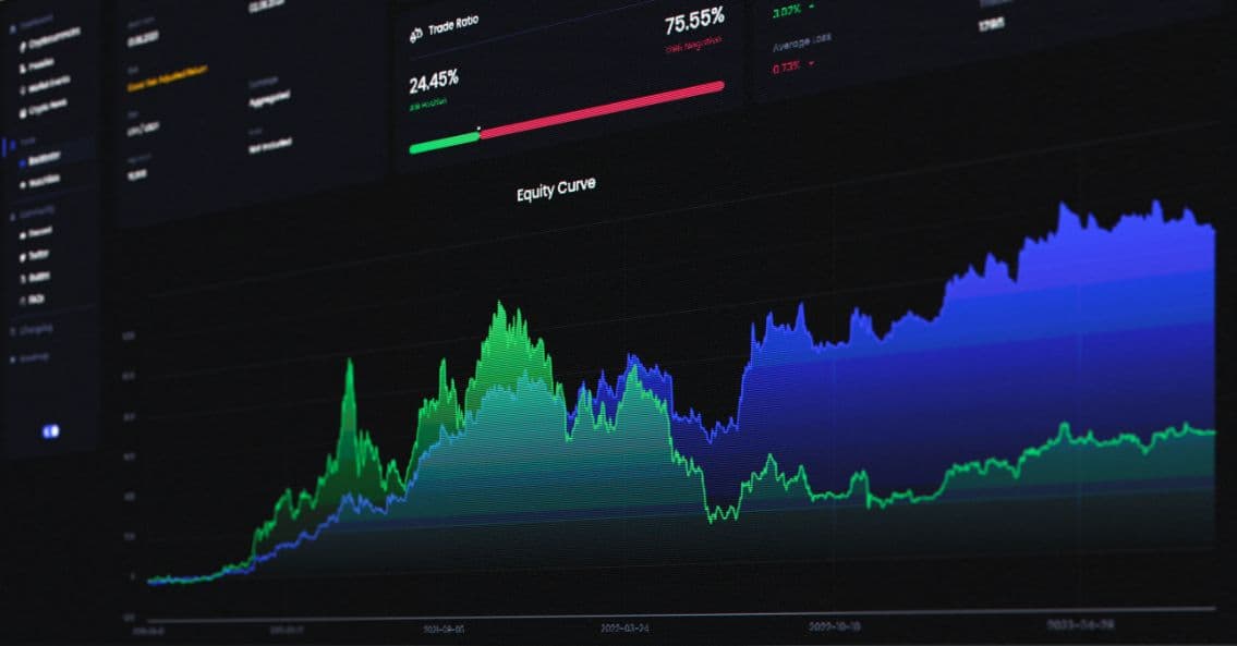
Trade Ratio: This metric indicates the percentage of winning trades and losing trades.
Trades Win/Loss:
- Average Win: It represents the average profit generated per winning trade.
- Average Loss: It reflects the average loss incurred per losing trade.

Interpreting Average Returns and Win Ratio
When considering the positive trade ratio against the average returns of a strategy, we can encounter several scenarios that provide valuable insights into its performance. Here are a few possible scenarios to consider:
High Profitable Trades Ratio with High Average Returns:
In this scenario, the strategy exhibits a high percentage of winning trades (positive trades ratio) along with a substantial average return per trade. This indicates a robust strategy that consistently generates profitable trades, resulting in significant overall returns.
High Positive Trades Ratio with Low Average Returns:
Here, the strategy has a high positive trade ratio but a relatively low average return per trade. This suggests that although the majority of trades are profitable, the magnitude of the profits may not be as substantial. The strategy may focus on frequent, smaller gains rather than large, infrequent wins.
Low Positive Trades Ratio with High Average Returns:
This scenario involves a lower percentage of winning trades (positive trades ratio) but a high average return per trade. Despite a relatively lower success rate, the strategy is capable of capturing significant profits when successful. It may rely on selective, high-reward opportunities that outweigh the losses incurred from unsuccessful trades.
Low Positive Trades Ratio with Low Average Returns:
In this scenario, both the positive trade ratio and the average return per trade are relatively low. The strategy struggles to generate consistent profits, with a significant portion of trades resulting in losses. This may indicate the need for further refinement or adjustments to improve the strategy's performance.
It’s important to assess the positive trade ratio in conjunction with the average returns to gain a comprehensive understanding of a strategy’s profitability. Each scenario provides unique insights into the strategy's strengths, weaknesses, and potential areas for optimization. By analyzing these factors, traders can make informed decisions to enhance their trading strategies and improve overall performance.
While a high percentage of winning trades may initially seem indicative of a successful strategy, it is crucial to consider additional factors to assess its overall performance. The average return per trade and average loss per trade provide deeper insights into the strategy's profitability and risk management.
A strategy with a high percentage of winning trades but a low average return may generate consistent profits, but the magnitude of those profits might be limited. Conversely, a strategy with a lower percentage of winning trades but a higher average return could yield substantial profits when successful trades occur. Therefore, it is essential to evaluate the balance between average returns and average losses, taking into account the risk-reward ratio and overall profitability. By considering these factors holistically, traders can make more informed decisions and develop strategies that align with their risk tolerance and profit objectives.
Charts
The Dash 2 Trade backtester results page features a number of charts that visualize key strategy success metrics.
Equity Curve
The equity curve graph visually displays the cumulative performance of the strategy over time compared to the performance of the target coin in a simple “buy and hold” strategy, allowing you to observe overall growth or decline for both.

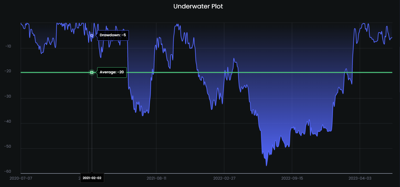
Underwater Plot (Drawdown)
This chart illustrates the strategy's drawdown, showing periods of losses and recovery. It helps assess the potential risk and magnitude of losses.
Heatmap Chart: Monthly Returns
The heatmap chart provides a visual representation of the strategy's performance on a monthly basis. It helps identify patterns and seasonal variations in returns.

Rolling Sharpe Chart
This chart calculates the rolling Sharpe ratio, which measures the risk-adjusted returns of the strategy over a specific period. It assesses the consistency of returns.

Rolling Sortino Chart
Similar to the rolling Sharpe ratio, the rolling Sortino ratio evaluates the risk-adjusted returns, focusing specifically on downside risk.

Rolling Volatility Chart
This chart displays the rolling volatility of the strategy and the target asset, providing insights into the correlation between the strategy and the target.

Rolling Beta Chart
The rolling beta measures the strategy's sensitivity to changes in the returns of a target asset. It helps assess the strategy’s correlation with the broader market.

Tables
In addition to the illustrative charts, there are numerous additional datapoints you can analyze, presented in a series of tables.
Overview

This table presents a set of metrics that provide valuable insights into the performance and characteristics of a trading strategy. These metrics offer a snapshot of key indicators such as cumulative return, annual growth rate, drawdown, risk measures, and more. Understanding these metrics helps traders assess the profitability, risk profile, and overall effectiveness of their strategies. Here is a simplified explanation for some of them:
- Avg. Up Month: This metric tells you the average amount of money the strategy made during months when it was profitable.
- Avg. Down Month: This metric tells you the average amount of money the strategy lost during months when it wasn’t profitable.
- Avg. Drawdown: This metric tells you the average amount of money the strategy lost from its highest point to its lowest point during losing periods.
- Avg. Drawdown Days: This metric tells you the average number of days it took for the strategy to recover from losses and reach a new high after a losing period.
- Recovery Factor: This metric compares the total amount of money gained by the strategy to the total amount of money lost. A higher value means the strategy is better at recovering from losses.
- Ulcer Index: This metric measures how large and how long the losing periods were for the strategy. A lower value indicates less severe losses.
- Serenity Index: This metric shows the percentage of positive periods (months, quarters, or years) within the total period. A higher value means the strategy consistently generated profits.
- Payoff Ratio: This metric compares the average profit made per trade to the average loss incurred per trade. A higher ratio means the strategy has a better balance between risk and reward.
- Profit Factor: This metric compares the total profit made by the strategy to the total losses incurred. A higher value means the strategy is more profitable overall.
- Expected Daily, Monthly, and Yearly Returns: These metrics estimate the average returns you can expect from the strategy on a daily, monthly, and yearly basis.
- Kelly Criterion: This metric helps determine the optimal amount of money to invest in the strategy based on its historical performance and risk level.
- Risk of Ruin: This metric calculates the probability of the strategy losing all of its invested capital or reaching a predefined threshold of losses.
- Tail Ratio: This metric measures the difference between the average returns during positive periods and the average returns during negative periods. It indicates the skewness of the strategy's returns.
- Daily Value-at-Risk: This metric estimates the maximum potential loss the strategy may experience on a daily basis, at a certain confidence level.
- Expected Shortfall (cVaR): This metric estimates the average loss that may occur beyond the Value-at-Risk threshold. It provides additional information about the potential magnitude of losses.
Risk
The Risk tab presents various metrics that assess the risk-adjusted performance and efficiency of a trading strategy. These metrics provide insights into the strategy’s ability to generate returns relative to the level of risk taken. Understanding these metrics helps traders evaluate the risk-reward tradeoff and make informed decisions about their investment strategies.

- Sharpe: The Sharpe ratio measures the risk-adjusted return of an investment. A higher value indicates better risk-adjusted performance.
- Prob. Sharpe Ratio: This metric represents the probability that the Sharpe ratio is greater than zero, indicating the likelihood of positive risk-adjusted returns.
- Sortino: The Sortino ratio evaluates the risk-adjusted return, focusing specifically on the downside risk or volatility. A higher value implies better risk-adjusted performance with respect to downside deviation.
- Smart Sortino: Similar to the Sortino ratio, the Smart Sortino ratio assesses the risk-adjusted return, taking into account downside risk. It considers a more refined downside deviation calculation.
- Sortino/√2: This metric is the Sortino ratio divided by the square root of 2, providing a standardized value for easier interpretation and comparison.
- Smart Sortino/√2: Similar to Sortino/√2, this metric is the Smart Sortino ratio divided by the square root of 2, allowing for standardized interpretation and comparison.
- Omega: Omega is a risk-adjusted performance measure that considers both upside and downside deviations. A higher value indicates better risk-adjusted performance.
- Common Sense Ratio: The Common Sense Ratio evaluates the risk-adjusted return by considering the downside risk. It assesses the returns relative to the average loss magnitude.
Metrics
This part compares different metrics for both a trading strategy and a buy-and-hold approach. These metrics provide valuable information about the strategy’s risk, performance, and distribution characteristics, enabling traders to assess its effectiveness compared to a passive investment strategy. Through the analysis of metrics like volatility, Calmar ratio, skewness, and kurtosis, traders can evaluate the strategy’s risk profile, risk-adjusted returns, and distribution properties in relation to a buy-and-hold approach.
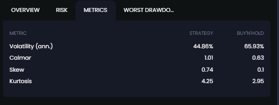
- Volatility (ann.): Volatility measures the degree of fluctuation or variability in the strategy's returns. Higher volatility indicates larger price swings and potentially higher risk.
- Calmar: The Calmar ratio assesses the risk-adjusted return by dividing the average annual return by the maximum drawdown. A higher value indicates better risk-adjusted performance relative to the drawdowns experienced.
- Skew: Skewness measures the asymmetry of the strategy's return distribution. Positive skewness indicates a tendency for larger positive returns, while negative skewness suggests a higher frequency of larger negative returns.
- Kurtosis: Kurtosis quantifies the shape of the strategy's return distribution. A higher kurtosis value indicates a distribution with fatter tails and potentially more extreme returns.
Final Comments
In conclusion, understanding and interpreting the general overview, charts, and tables in backtesting results is crucial for evaluating trading strategies. It is important to consider multiple factors and metrics to gain a comprehensive understanding of a strategy's performance. By analyzing metrics such as cumulative return, CAGR, win ratio, drawdown, and various risk metrics, traders can assess the profitability, risk profile, and consistency of a strategy.
Charts such as the equity curve, underwater plot, and heatmap provide visual representations of the strategy's performance over time, revealing trends, periods of drawdown, and the distribution of returns. These charts help traders identify strengths, weaknesses, and potential areas for optimization.
Tables, on the other hand, present numerical data and metrics that offer deeper insights into specific aspects of the strategy, such as risk-adjusted returns, volatility, skewness, and kurtosis. These metrics allow traders to analyze risk-reward ratios, assess the strategy's risk profile, and understand the shape and distribution of returns.
To make informed decisions, it is important to combine the analysis of multiple factors and metrics. Relying on a single metric or chart may provide a limited perspective. By considering various metrics and charts together, traders can gain a more holistic view of the strategy's performance and make informed decisions about its suitability for their trading objectives.
Ultimately, the goal of using combined analysis is to identify strengths and weaknesses, refine trading strategies, and improve overall performance. Regularly reviewing and analyzing backtesting results using multiple factors helps traders adapt and optimize their strategies in response to changing market conditions and dynamics. It is an iterative process that requires continuous monitoring, evaluation, and adjustment to stay ahead in the dynamic world of trading.